dhmin: Mathematical optimisation model for district energy distribution networks
| Maintainer: | Johannes Dorfner, <johannes.dorfner@tum.de> |
|---|---|
| Organization: | Chair of Renewable and Sustainable Energy Systems, Technical University of Munich |
| Version: | 0.1 |
| Date: | Sep 27, 2017 |
| Copyright: | The model code is licensed under the GNU General Public License 3.0. This documentation is licensed under a Creative Commons Attribution 4.0 International license. |
Contents
Features
- dhmin is a mixed-integer linear programming model for single-commodity energy distribution networks.
- It finds the minimum cost (invest + operation - revenue) energy distribution network for a given set of energy source locations (source vertices) and a set of demand locations (possible customers).
- Temporal resolution is variable, but incurs a strong limit on the feasible spatial resolution. I.e. with about 2-3 timesteps, hundreds or several thousand edges are possible in reasonable time.
- Thanks to pandas and GeoPandas complex data analysis code is short and concise.
- The model code itself is very short thanks to relying on the Pyomo package.
- The model code is structured identical to the more general urbs model.
Screenshots
This is a typical result plot created by function dhmintools.plot_flows_min for the accompanying minimal example dataset. There are (not shown) two demand edges (with x,y coordinates [5,7 to 4,9] and [7,2 to 6,3]) in this graph. Three possible source vertices (red dots) with sufficient capacity are located at the vertices with coordinates [2,2] [2,7] [9,9] and feature different generation costs, [9,9] being cheaper than the other two.
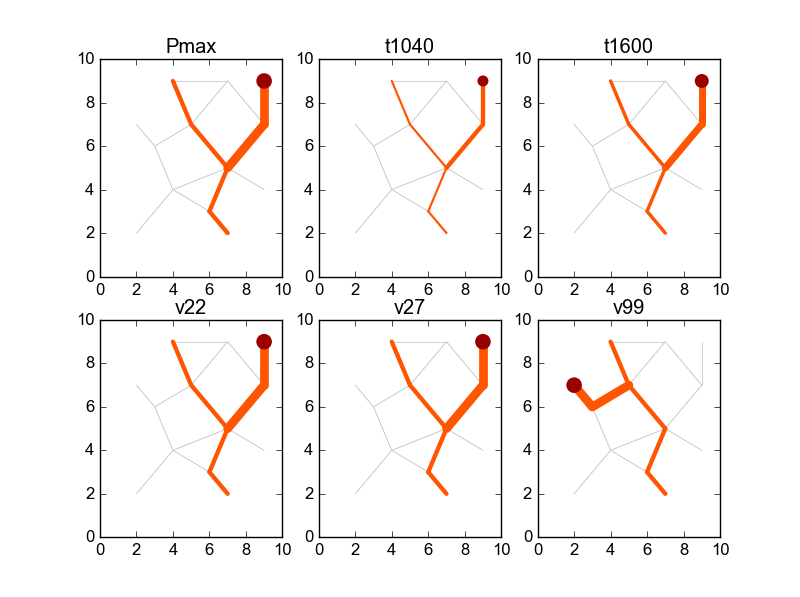
The first subplot Pmax shows the power flow from the cheapest source vertex (north east) to the two demand locations, indicating that both locations can be connected economcially. The two plots t1040 and t1600 show the minimum-cost power flow configuration for the provided partial load situations.
The second row shows the power flow configuration that occur when outages of the source vertices occur. As only vertex [9,9] is used exclusively anyway, only its outage (last plot) changes the
The built pipe capacity and layout is planned so that a) satisfying all profitable demands at minimum costs and b) that all pre-determined contigency situations can be handled with the constructed capacities.
Dependencies
- Python versions 2.7 or 3.x are both supported.
- pyomo for model equations and as the interface to optimisation solvers (CPLEX, GLPK, Gurobi, ...). Version 4 recommended, as version 3 support (a.k.a. as coopr.pyomo) will be dropped soon.
- pandas for input and result data handling, report generation
- Any solver supported by pyomo (GLPK, CBC, CPLEX, Gurobi, ...)